The Voter Model Simulation

Table of Contents

Mathematical Details

In this article, I will go into the program I wrote to simulate the voter model. If you are interested in how the voter model is defined, you can read the article I have written about it.

Graphical User Interface (GUI)

I decided to implement the simulation on flat-tori in one and two dimensions. That just means that, in one dimension, we have nodes that are set up in a row and each node connects to its left and right neighbors and the node at the beginning of the row is connected to the node at the end of the row. In two dimensions we have a by grid and each node is connected to its four neighbors, top, bottom, left and right, with the nodes at the bottom row connecting up to the top and similar for those at the left.

Simulation I

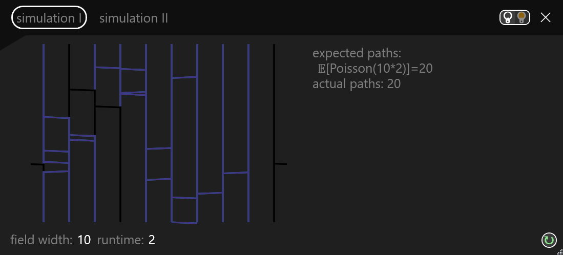
We also have a time dimension, since the nodes change state over time, on the one-dimensional torus I chose to visualize time as another axis, downwards.

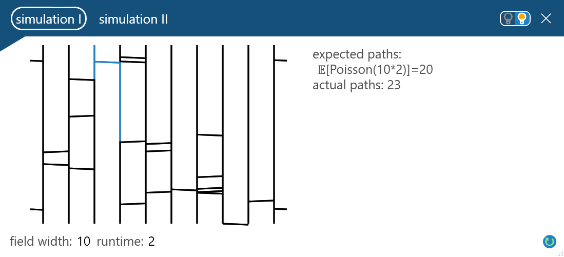
We can see the simulation on the left and some details about the probabilities on the right. The jump times are the times at which one node adapts the opinion of another. Since the jump times are the times at which a Poisson process “ticks” we can get the number of jumps on average by taking the expected value of a Poisson distributed variable with rate time times number of edges. In our case, the number of edges is equal to the number of nodes and the time is the time we decide to let the simulation run. Finally, the expected value of a Poisson distributed value is its rate, which is what we read under “expected paths” on the right side in the picture above.

In my program, field width and runtime are adjustable and we can get another simulation by clicking the refresh symbol at the bottom right.

Simulation II

The second simulation does not show the time axis but just runs in real-time and we can see the current state of the grid in the display.

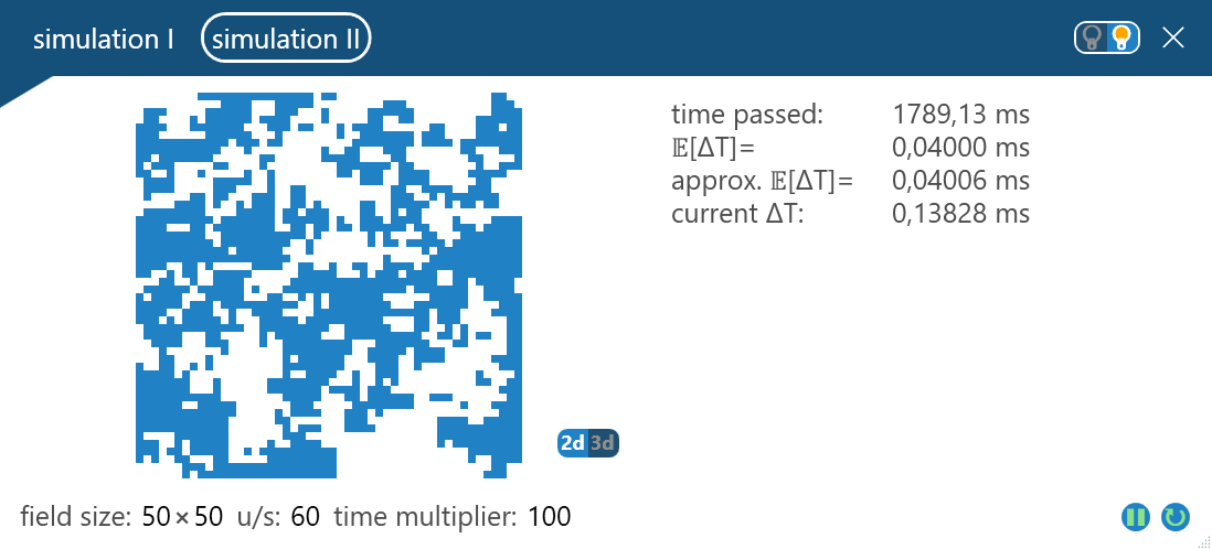
On the right, we have some data about the simulation again. We can see how much time has passed since the beginning, as well as the expected timespan between jumps. This timespan is exponentially distributed with rate one over the number of nodes. We can also see the approximated timespan between jumps, it is calculated by tracking the actual timespans between jumps and dividing them by the number of jumps so far. The current is the last timespan between jumps.

We can adjust the size of the field as well as the updates per second “u/s”, which is comparable to fps. The time multiplier setting controls how fast the simulation runs. In this case the average timespan between jumps is we use the time multiplier to “convert” this number to milliseconds .

Since the field is on a 2d torus I have also implemented a vies that maps the graph onto a spinning torus:

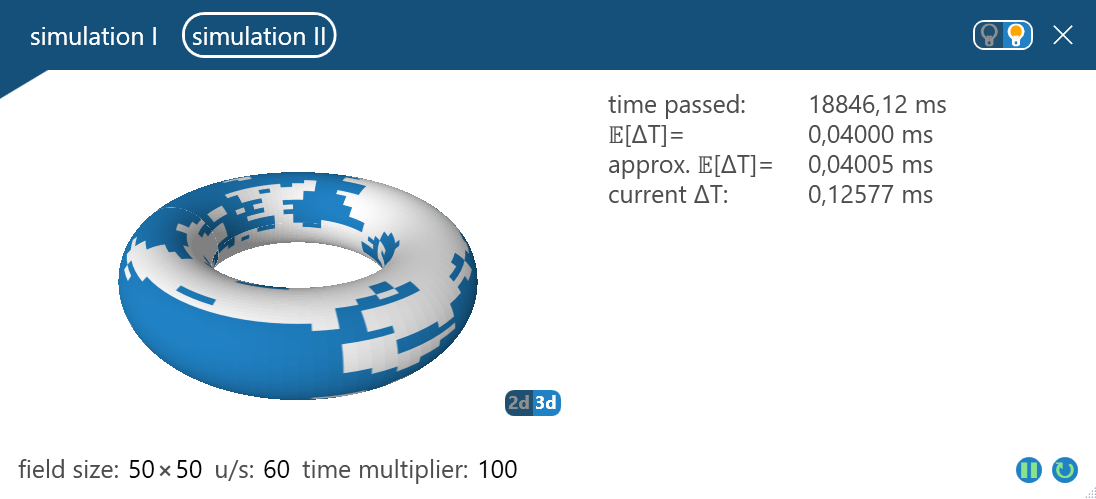
We can pause or reset the simulation by using the buttons on the bottom left. Additionally, I have implemented a dark mode, which we can toggle on at the top left.

Implementation

The implementation is also different for the two simulations since we can run the first simulation until the specified time and then display the result in full. The second simulation needs to run in real-time and thus we need a continuously called update function and then update the graph based on the changes in this function.

Simulation I

We define a function called “RunUntilAfter” that takes the time until the simulation is run. In every iteration of the loop, we realize the time passed randomly from an exponential distribution and select the place to which the jump happens uniformly and the neighbor from which the jump happens also uniformly. We also need to make sure that the first and last node are connected, which we do by adjusting the index of the neighbor if it is outside the valid index range.

The time passed is called “deltaTime” and “Length” is the size of our graph.

/* ... */ RunUntilAfter(double endTime)
{
  /* ... */
  double timePassed = 0;
  while (timePassed < endTime)
  {
    double deltaTime = RandomVariable.Exponential(Length);
    int randomPlace = RandomVariable.UniformDiscrete(Length);
    int randomNeighbor = randomPlace + (2 * RandomVariable.UniformDiscrete(2) - 1);

    if (randomNeighbor == Length)
        randomNeighbor = 0;
    else if (randomNeighbor == -1)
        randomNeighbor = Length - 1;

    /* ... */
  }
  /* ... */
}

This function should return the graph at all jumping times, so we return a list of graphs and timestamps for rendering. We also need to advance the time passed and lastly, we just need to make the selected nodes adapt their selected neighbor’s opinion.

List<Graph, double> RunUntilAfter(double endTime)
{
  List<Graph, double> GraphOverTime = new List();
  GraphOverTime.add(Graph.RandomState(Length), 0);

  double timePassed = 0;
  while (timePassed < endTime)
  {
    timePassed += deltaTime;

    double deltaTime = RandomVariable.Exponential(Length);
    int randomPlace = RandomVariable.UniformDiscrete(Length);
    int randomNeighbor = randomPlace + (2 * RandomVariable.UniformDiscrete(2) - 1);

    if (randomNeighbor == Length)
        randomNeighbor = 0;
    else if (randomNeighbor == -1)
        randomNeighbor = Length - 1;

    var currGraph = GraphOverTime.Last()[0].Copy()
    currGraph[randomPlace] = currGraph[randomNeighbor]
    GraphOverTime.add(currGraph, timePassed);
  }

  return GraphOverTime;
}

For the implementation of the Graph type, we can use an array:

public class Graph
{
  private bool[] Nodes;

  public bool this[int key]
  {
    get => Nodes[key];
    set => Nodes[key] = value;
  }

  public Graph(bool[] nodes)
  {
    Nodes = nodes;
  }

  public Graph Copy()
  {
    var nodesCopy = new bool[Nodes.Length];
    Array.Copy(Nodes, nodesCopy, Nodes.Length);
    return new Graph(nodesCopy);
  }

  public static Graph RandomState(int length)
  {
    var nodes = new bool[length];
    for (var i = 0; i < length; i++)
    {
      nodes[i] = (bool)RandomVariable.UniformDiscrete(2);
    }
    return new Graph(nodes);
  }
}

For the RandomVariable type, we can get all the values we need from a function that can return a random number in the unit interval e.g. new Random.NextDouble(). Note that you should not have too many instances of the Random class. We will assume that the function rand() is some implementation of this function.

public class RandomVariable
{
  public static double Exponential(float rate) {
    var r = rand()
    while (r == 0)
      r = rand()

    return -Math.Log(r / rate) / rate;
  }

  public static int UniformDiscrete(int max /*excluded*/) {
    return (int)Math.Floor(rand() * max);
  }
}

Simulation II

The main difference in this simulation is caused by displaying the change in real-time. Concretely this means that instead of having a function that just runs a loop until the time is up, we have a “Next” function that is called indefinitely. Otherwise, we are doing the same thing: pick a node, pick a neighbor, get the time passed, and update the graph.

public class Simulation2d {

public Graph2d Graph;
public float TimeMultiplier;

public void Next()
{
  randomPlaceRow = RandomVariable.UniformDiscrete(Width);
  randomPlaceCol = RandomVariable.UniformDiscrete(Height);

  randomNeighborRow = randomPlaceRow + (2 * RandomVariable.UniformDiscrete(2) - 1);
  randomNeighborCol = randomPlaceCol + (2 * RandomVariable.UniformDiscrete(2) - 1);

  deltaTime = RandomNumberGenerator.RealizeExponentialRandomVar(Height * Width);

  if (randomNeighborRow == Width)
        randomNeighborRow = 0;
    else if (randomNeighborRow == -1)
        randomNeighborRow = Width - 1;
  
  if (randomNeighborCol == Height)
        randomNeighborCol = 0;
    else if (randomNeighborCol == -1)
        randomNeighborCol = Height - 1;

  Graph[randomPlaceRow][randomPlaceCol] = Graph[randomNeighborRow][randomNeighborCol];
  return deltaTime;
}

public void Start() {
  Graph = Graph2d.RandomState(Length);
  var currTime = Time.Now();
  Display.Draw(Graph);

  while(True) {
    var timePassed = 0
    while(timePassed * TimeMultiplier < Time.Now() - currTime) {
      timePassed += Next();
    }

    var currTime = Time.Now();
    Display.Draw(Graph);
  }
}

}

The “Start” method initializes the graph randomly and then starts calling “Next” and “Display.Draw”, it also keeps track of when the last drawing happened, so we can always only call “Next” until we are caught up with the actual time that passed. Additionally, we have the “TimeMultiplier” that converts the time passed in the simulation into real-time. Let us say “Time.Now” returns the time passed since the program started in milliseconds, then “Time.Now() - currTime” in the loop is the time since the last drawing in milliseconds, for TimeMultiplier that means that ms are the equivalent of unit of simulation time. The class “Graph2d” is similar to “Graph”, so I wont go into detail about it.

Checking Probabilities

We can check that RandomVariable.Exponential() has the right distribution:

We in the proof above we assume that but actually is -distributed and then redrawn if . But this is also not correct, in reality, a computer can only represent a finite countable amount of numbers between so let us call the set of numbers our computer can represent . Since those numbers are countable and finite we can number them from one to , .

We also need to consider that these numbers in are not equidistant. For example if we would have for . Which does not look like a -distribution. So we potentially need to distribute the values in , such that and . Let us call this distribution .

Next, we want to model redrawing until the first non-zero value. Consider:

Then is the variable we are interested in:

First for :

The first and last equality follow by definition and the second by independence of .

Now :

We have every part of our original sum in a usable state now, the last step is to do the summation:

This is the result we expected, is distributed such that it only takes values in with probability respectively. Which approximates . If we did not have to do the redistributing, maybe because the values in are equidistant, we would have for all , this makes our result much more intuitive:

and

This means the distribution changes from picking uniformly among elements to picking uniformly among elements which is exactly what we are doing by leaving out the zero.