Introduction
Table of Contents
Motivation
In this article, I will try to give an introduction to statistics and a general intuition about how to use and interpret commonly seen concepts like p-values, significance levels and confidence intervals. I will focus on applying statistical methods rather than proving related theorems. This article often references Geo2015(German). I have also written a follow-up article in which I go deeper into parameter estimation and have more information about the interpretation of these concepts.
Random Variables and Observations
Whenever we want to apply statistical methods we need observations, meaning we need to measure some values. Whenever we want to make theoretical statements about the underlying laws of statistics we need to consider what generates these observations.
Consider a dice, we can roll the dice and look at the number it lands on, this number is the observation. The rolling is the way this observation is generated. If we had all the information about the the dice at the time of the roll we would be able to calculate on which number it lands on. So we have a function that takes the current state of the universe and outputs the result of the experiment. We call this function a random variable:
contains all states of the universe and is the input of , models the dice roll and the observation is a number in , for . For a more rigorous definition of random variables consider reading Geo2015 p.21ff.
We may be interested in a fair dice landing on a six. We can define where is the Bernoulli-distribution. is either zero or one and models the dice landing on a six or not respectively. We can say the chance of a six is one in six:
If we roll a six we observe .
We are not interested in the mathematical details of and we will often omit it entirely. This is reflected in our notation, above we wrote . means . Rather we will look at the distribution of the random variable, e.g. how likely it is for the random variable to have some value.
But why is this distinction important? In the following chapter, we will be using several observations to calculate the mean of all observations. We then want to show that this empirical mean is in some sense close to the actual expected value of the underlying distribution. Or more generally we want to show that we can approximate parameters, like expected value, variance or moments of a distribution by only using observations we have measured.
For the empirical mean, we show that for all states of the universe that we plug into the random variables they have an empirical mean equal to the excepted value. This means that calculating the mean of the observations is a sensible thing to do that gives us an estimation of the expected value.
Mean and Variance Estimation
Let be independent identically distributed (iid) random variables for some distribution and some observations. We write , for our random vector and observation vector respectively.
As an example let the Poisson-distribution where would be the expected value . This is unknown and we want to estimate it, based on the observations . The first intuition we might have is to compute the empirical mean value of our observations:
Mean Estimation
To see if this is a good idea we might want to look at the expected value of the estimator :
The property of the expected value of the estimator being equal to the value that is supposed to be estimated is called unbiased: is an unbiased estimator of the mean. By the law of large numbers (LLN), we know that . By definition, this means:
so
where . We will not go into the meaning of here and instead heuristically focus on
In stochastics we often omit , but remember that
So for (almost) all the empirical mean of the observations will be close to if is large. We say almost all since might not be the empty set.
This is good news and can be interpreted as: if we have enough observations the empirical mean will go towards the actual mean of our distribution. Notice that we did not use the Poisson distribution to arrive at this result. We can further generalize this result: for iid., we can use to estimate . Specifically for we can estimate the mean of our distribution by calculating .
Variance Estimation
We can do the same for the variance which we will also need later:
We can also show that :
since and , the assertion follows.
The general concept of this idea is called parameter estimation. We will look at an example of parameter estimation in the follow-up article about this topic, which shows that we might want to choose a different estimator than to approximate the parameters of a distribution.
T
We can combine and in a useful way that we can use when talking about confidence levels and hypothesis tests, for this, consider iid. random variables with mean and variance , then set:
We have shown that , so by the central limit theorem , converges to a normal distribution in distribution, which means:
In case of iid. we know the distribution of exactly: the (Student’s) -distribution. For a prove of this see Geo2015 p.277ff.
This will be very useful in the following chapters. For now just notice the difference here: in general we know that converges in distribution to a normally distributed variable but for we know the distribution exactly and do not need to use convergence.
Hypotheses Testing and Confidence Intervals
Motivation: Plausibility Rather than Truth
In statistical analysis, we are not able to say anything with certainty. Meaning we cannot make statements about something being true or false. Rather we have to focus on making conclusions about whether something is plausible based on the data we are presented with.
We can think about one thing affecting something else, like, how medication could affect how severe the patient’s illness is. Then we come up with a zero hypothesis that denies the effects, our test aims to reject this zero hypothesis. For medication, we aim to show that it is implausible that there is no effect from medication on the severity of illness.
Recognize this pattern from proofs by contradiction: in that case, we would show that we arrive at a contradiction if we assume what we are trying to prove is false. Then we can conclude that what we are trying to prove is true. One popular example of a proof by contradiction is the existence of infinitely many prime numbers.
To Show: There are infinitely many prime numbers.
Proof: Assume that there are in fact, finitely many prime numbers . Then consider the number . is not divisible by any of the numbers but is also not equal to any . Thus since we know every number has a prime factorization, we know that our original assumption is false: there are not only finitely many primes!
This is similar to the method we would apply in statistics, we come up with a zero hypothesis that we show to be implausible. In this example, the zero hypothesis would be that there are finitely many primes. Unlike proofs of contradiction however, we would not be able to show that a zero hypothesis is false, just that by assuming the zero hypothesis, the data we have collected is relatively unlikely to occur, so we conclude that our zero hypothesis must not be plausible.
In the chapter Type I and Type II error we will see that we can either exactly limit how often we falsely reject or how often we falsely do not reject the zero hypothesis and that we implicitly limit the other as well if we choose the one we limit. Conventionally, the zero hypothesis is chosen such that falsely rejecting it is limited exactly and that that is better than falsely not rejecting it. For in a medical trial, we would set the zero hypothesis to be the medication having no effect. Since distributing potentially harmful medication to unsuspecting patients is worse than falsely believing that the medication is useless.
Hypothesis Testing
A common statistical question is, to gain some insight about an unknown parameter of a distribution. Imagine we publish some program we made online, we can track its downloads within the next week and decide we will publish an update if the program becomes popular enough. The Poisson distribution is a good model distribution in this case since it is a discrete, positive distribution that has all its mass around its mean, just like we would think of the number of downloads of a program. We find more than downloads in a week to be sufficiently popular.
So the question is, is ? As discussed before we want to show that the opposite statement is not plausible and we call this statement the zero hypothesis: .
Now what does it mean for data to be implausible? Let us assume we have a random variable, we can calculate the chance of this random variable being bigger than some :
If we have an observation , we would say it is implausible that this was generated by a Poisson distribution with if it is very large. Just like we would think rolling a six on a dice 20 times in a row makes it very implausible that this dice is fair.
In concrete terms, we want to find a maximum value for our observation that is not implausible to get in the situation of the zero hypothesis. To find this highest still plausible number we set a significance level that is bigger than the maximum probability of observing a higher value than . Thus is defined in the following way.
If the actual observation then is bigger than it is implausible that this is from a Poisson distribution with . We can reject the zero hypothesis.
Often is set to and in this case is rising in so . The formula for simplifies to:
To get all we need to do now is to calculate the probabilities until we find the one that matches the formula. In the table below we see that is the first probability to be smaller than , so is one bigger than the last plausible value: . We reject if ! For a short discussion of the choice of , read this chapter.
Let us generate a few observations from different Poisson distributions in python:
import scipy.stats as st
import numpy as np

np.random.seed(234)
observations = [
  st.poisson.rvs(mu=90),
  st.poisson.rvs(mu=100),
  st.poisson.rvs(mu=101),
  st.poisson.rvs(mu=110),
  st.poisson.rvs(mu=150),
]
print(observations)
As the output we get [105, 92, 114, 109, 158], and reject for the last observation, meaning we would consider it to be implausible that this observation is generated by a Poisson distribution with an expected value smaller than .
The third and fourth observations are also generated by a Poisson distribution with . However, we cannot reject in these cases based on our observations. This is a general problem with checking plausibility rather than absolute truth, we might consider something to be plausible even though the unknown underlying reality disagrees.
Let us quickly summarize our approach:
- Choose a parametrized distribution and a parameter space for the data that is appropriate for the observations we generate: e.g. for
- Seperate into zero Hypothesis and alternative: e.g.
- Choose an significance-level for what is plausible under , commonly
- Pick a statistic . For reject otherwise do not reject e.g.
- Make an observation , if we can reject
Be careful to accept if the observation is plausible, we are only making sure that under it would be plausible but we are not doing anything to test if it would be implausible in the alternative case, meaning the observation might also be plausible in the alternative case. We can swap the zero Hypothesis and the alternative in our example and find for an alpha level of that the smallest still plausible observation of our previous alternative is . For the previous observations [105, 92, 114, 109, 158] that means we can consider them all plausible in the alternative !
We now have four possible situations:
| is true | is true | |
|---|---|---|
| rightfully not rejecting | falsely not rejecting | |
| falsely rejecting | rightfully rejecting |
We obviously do not want to falsely reject or falsely not reject, the former case is controlled by our : . So we only need to think about the second case, in the next chapter, we will introduce some definitions to talk about these errors better and find that we have to make a trade-off between the former and the latter error.
Type I and Type II error
Let us look at the expected value of the statistic ,
We call this the Goodness Function which I chose to translate from German after being unable to find a translation that is commonly used. Also see Geo2015 p.289.
In our example . We say our test has significance level if
We chose for a significance level of in the example. is called Type I error for , the probability of rejecting even though is true. So is the Type I error in the worst case. The type II error is for , the probability of not rejecting even though the alternative is true.
Intuitively we can see that we want both of these errors to be small, for this, we might choose a very small . In our example, we have the maximal type II error:
So for small the maximal type II error is large, which we wanted to avoid. This is often the case. For this simple setup, we have arrived at this result by merely using monotony of . This means we are doing a trade-off between type I and type II errors.
If we look back again at our generated observations from before we can plug in and calculate the type II error in those cases. The type II errors for the cases are , respectively. So in the case of , we (falsely) do not reject in of cases! In literature for is also often called power of a test: for “close” to the test has little power.
We might ask why the goodness function is an expected value rather than just being the probability of rejecting ? In our case this would not make a difference since we are using statistics that are either zero or one. In general however we might be testing something regularly and want to match the significance level exactly e.g. . In this case we can construct a decision rule that takes a third value , now the goodness function becomes and we can choose gamma to match the significance level exactly.
The immediate follow up question is: what do we do if is equal to for our observations, if it was one we rejected and if it was zero we did not reject. If we perform an independent random experiment that takes values zero and one with probability of the result being one equal to . Then we reject if we got a one.
This may seem counterintuitive. Why are we now deciding based on random chance? But notice we only use random chance for certain constallation of observations and by doing so we can exactly control the worst type I error of our test which means we control how much we maximally erroneously reject our zero hypothesis. See Geo2015 p.287ff & p.292ff for more information.
Approximate Testing with the Central Limit Theorem
First, we introduce quantiles:
Quantiles
We define the -quantile of a distribution such that, for :
If our distribution is continuous we can say equivalently:
For the -distribution, we will call the -quantile and for the standard normal distribution . Note that the quantiles of the -distribution converge towards the quantiles of the normal distribution for large , as one would expect.
In the continuous case, we see that a quantile is the inverse function of the distribution function.
Imagine now we have random variables iid. with and want a to do a test , we know:
From the convergence properties of we also know: . For an independent random variable.
So we get a test that approximately has significance level , for a large sample size:
Since this is an approximate method we might want to simulate it for a few distributions and see how well it works when implemented. I am using the following imports.
import scipy.stats as st
import numpy as np
import matplotlib.pyplot as plt
First, we need to implement a function that approximates , for a given distribution of the observations. We can do this by supplying the function with the information it needs to realize observations and calculate . That is the distribution and , as well as how many observations we have made: “observation_count”. For simplicity’s sake, we want all the distributions, we supply to have the same expected value which we achieve by additionally adding the expected value “mu” to the function. Then we just need to subtract the distribution mean from the observation and add mu.
Then we just calculate for several observation sets, in this case and calculate the empirical chance of it being larger than the quantile z.
def empirical_probability(m_0, mu, observation_count, distribution):
  alpha = 0.1
  repetitions = 100
  z = st.norm.ppf(1 - alpha)

  prob = 0
  for _ in range(repetitions):
    mean = distribution.stats(moments='m')
    observations = distribution.rvs(size=observation_count) - mean + mu
    emp_mean, emp_var = np.mean(observations), np.var(observations)
    S = (emp_mean - m_0) * np.sqrt(observation_count / emp_var)
    prob += S > z
  prob = prob / repetitions
  return prob
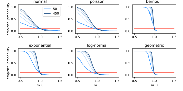
Next, we pick the distributions and setup the plots, we pick a range of mu_0 to see what values we estimate for different choices of m_0, the expected value of the distributions is mu and set to here. If we run this we expect a curve that is almost at the beginning then drops to around and stays there. Since if m_0 < mu the zero hypothesis is rejected and thus which should be the case as long as m_0 < 1.
distributions = np.array([
  st.norm.freeze(loc=10, scale=4),
  st.poisson.freeze(mu = 10),
  st.bernoulli.freeze(p = 0.8),
  st.expon.freeze(),
  st.lognorm.freeze(s = 1),
  st.geom.freeze(p = 0.8),
])

fig, ax = plt.subplots(2, 3, figsize=(8, 4))
fig.tight_layout()
ax = np.array([ax]).flatten()

alpha = 0.1
observation_count = 50
mu = 1
m_0 = np.linspace(mu - 0.5, mu + 0.5, 30)
for i in range(len(distributions)):
  prob = empirical_probability(m_0, mu, observation_count, distributions[i])
  ax[i].plot(m_0, prob)
  ax[i].plot(m_0, alpha * np.ones_like(m_0))
Some details of the code for creating the plots have been omitted to keep the focus on the mathematical details
The y-axis of our graphs is m_0, the actual mean of the plotted distributions is mu and the zero hypothesis is mu m_0. So on the left half of the graph, the zero hypothesis is inaccurate and on the right it is accurate. At any point m_0 the plotted line describes the empirical probability of rejecting the zero hypothesis. As discussed before we would like the line to be on the left, not rejecting when it is true and on the right, rejecting when it is false.
Let us analyze the graphs in two steps, first consider the right side of the graph (m_0 > 1), where the zero hypothesis is accurate. We (falsely) reject about of the times for enough observations, which is the we set to be an acceptable amount of false rejections. However, in the case of the normal and Poisson distributions for a small number of observations, we reject more often - our test does not keep the set significance level!
We should have intuitively expected what we see here, for a small number of observations we should aim to get a better understanding of the distribution of our data and come up with a test tailored for this distribution, whereas for a large number of observations, the convergence has made our test sufficiently reliable.
Now consider the left side of the graph (m_0 < 1), where the zero hypothesis is inaccurate. We (rightfully) reject in this case, we find that the graphs are rising slowly to . This means we do not reject very frequently even though it is false. This is very interesting and explains why I avoided making statements about accepting the zero hypothesis: With we only control how frequently we falsely reject but not how frequently we falsely do not reject, not being able to reject should not mean that we accept it! We rather think it is plausible enough to be true, if we want to confirm the hypothesis we should collect new data and then conduct a new test where the zero hypothesis is the new alternative and vice versa.
We get similar approximative tests for and :
and
respectively, the derivation is similar to the first case and for the third case we also use the fact that the normal distribution is symmetrical, hence .
Note here that if our observations stem from a normal distribution and we have a small number of observations we can use the quantiles of the -distribution quantiles instead of the normal distribution quantiles and get better tests. (In some sense the best tests, see Geo2015 p.306ff.)
p-Value
The p-value is a simple way to see the significance of a hypothesis test. Normally we would check if the decision rule for our observations is one or zero and then reject the zero Hypothesis if .
For example, with our approximate test , this comes down to looking up , calculating , and then comparing the two values, if the latter is greater than the former we reject .
Instead, we could also calculate how likely it is to get a less plausible result under the zero hypothesis, meaning we could calculate
where are random variables of the distribution we assumed to be generating our observations.
In the case of normal distributed we know that , so with being the distribution function of the -distribution we know:
For other distributions and a large sample size, we can use the approximative normal distribution. With the distribution function of the standard normal distribution we calculate the p-value .
For the tests and , we would calculate
and
respectively. In the second case, the second equality follows from the symmetry of the normal distribution and since the -distribution is also symmetric we would have analogous formulas for the p-values in that case, but with the distribution functions of the -distribution instead of . We will look further into the p-value in the chapter p-Value interpretation of the follow-up article.
With the p-value, we can reject our zero hypothesis if , intuitively this makes sense: the p-value is the probability of getting a less plausible result than we have observed under the zero hypothesis, so if is smaller than it is less likely to get a less plausible result than the least plausible result to not reject as limited by .
As an example let us sketch the proof of
in the case . This means is equivalent to > rejecting :
For very large:
The last equivalence follows from monotony of probability measures.
Confidence Intervals
Often we are interested in estimating the mean of our data i.e. we assume that the underlying mechanic that produces our data has a certain distribution with finite mean and we want to approximate this mean and have some metric for how close the actual mean is to our approximation. For this, we will again use to create a confidence interval around .
To come up with a confidence interval we try to find such that, for a given small :
Then we could say: with high probability the interval includes the actual mean of our distribution. Since we have just shown, that the distribution of approaches normal distribution. We can approximate with the distribution function of the normal distribution and choose to be the -quantile of the normal distribution.
For the -quantile has the property .
This gives us a right-sided confidence interval for the mean and similarly, we can come up with a left-sided and centered confidence interval:
by noticing
and
In both equations, we can use , since the normal distribution is symmetrical.
In summary, we have come up with the following three approximate confidence intervals for level and the -quantiles of the normal distribution:
Remember that these are only approximate intervals since is only asymptotically normally distributed. Next, we will take a quick look at a case in which we know the actual distribution of .
Again in the case of observations from a normal distribution, we can use the quantiles of the -distribution, other than that the formulation of the confidence intervals remains the same. For small we get tighter confidence intervals if we do so.
We can also directly connect the p-value of the approximate test and the approximate centered confidence intervals, which we often get when we test whether or not two groups have the same mean, e.g. in A/B testing. We show that we can reject the zero hypothesis if is not within the confidence interval, here.
Summary
In this article we have come up with commonly used estimators for the mean and variance as well as the value:
- .
We have established how to come up with hypothesis tests and used the estimators above to construct approximate statistic functions for rejecting the zero hypothesis:
- ,
additionally, we have found the p-values for these tests, and we have shown that a p-value smaller than means we can reject the zero hypothesis:
Lastly, we have constructed approximate confidence intervals for the mean of the datas distribution:
For a deeper insight into parameter estimation, a discussion of what significance level should be used and common pitfalls of interpreting the p-value as well as an interesting connection between the p-value and confidence intervals, read the next article in this series.